DEVELOPMENT OF STREAMFLOW DROUGHT INDICES IN THE MORAVA RIVER BASIN  

Ondrej Ledvinka, Pavel Coufal 

Czech Hydrometeorological Institute 

Corresponding author: Ondrej Ledvinka, Czech Hydrometeorological Institute, Hydrology Database and Water Budget

Department, Na Sabatce 2050/17, 143 06, Prague 412, Czechia, ondrej.ledvinka@chmi.cz

ABSTRACT

The territory of Czechia currently suffers from a long-lasting drought period which has been a subject of many studies, including the hydrological ones. Previous works indicated that the basin of the Morava River, a left-hand tributary of the Danube, is very prone to the occurrence of dry spells. It also applies to the development of various hydrological time series that often show decreases in the amount of available water. The purpose of this contribution is to extend the results of studies performed earlier and, using the most updated daily time series of discharge, to look at the situation of the so-called streamflow drought within the basin. 46 water-gauging stations representing the rivers of diverse catchment size were selected where no or a very weak anthropogenic influences are expected and the stability and sensitivity of profiles allow for the proper measurement of low flows. The selected series had to cover the most current period 1981-2018 but they could be much longer, which was considered beneficial for the next determination of the development direction. Various series of drought indices were derived from the original discharge series. Specifically, 7-, 15- and 30-day low flows together with deficit volumes and their durations were tested for trends using the modifications of the Mann– Kendall test that account for short-term and long-term persistence. In order to better reflect the drivers of streamflow drought, the indices were considered for summer and winter seasons separately as well. The places with the situation critical to the future water resources management were highlighted where substantial changes in river regime occur probably due to climate factors. Finally, the current drought episode that started in 2014 was put into a wider context, making use of the information obtained by the analyses.

Keywords: climate change, nonstationarity, stochastic processes, statistical hydrology, Moravia

INTRODUCTION

The current long-lasting drought period in Czechia has steered the attention of the public and many scientists to the question whether climate change is responsible for the origin of such a situation. Indeed, according to Šercl et al. (2019), the beginning of the period dates back to the winter 2013/2014 which was characterized by less amount of snow cover and higher air temperature. During the next months, the combination of prevailing lack of precipitation and above-normal air temperature did not help overcome the adverse conditions where even groundwater recharge was lowered, which, in turn, influenced also the amount of water in rivers, and the phenomenon known as streamflow drought developed. The water deficit has not been compensated even though some of the next winters were again rich in snow. Despite the presence of several water reservoirs in Czechia, some parts of it have suffered from the water shortage affecting various sectors of economy including agriculture and water supply (e.g., Ledvinka, 2015a), which, incidentally, was the main impulse to establish inter-ministerial bodies addressing the issues connected with drought, and to financially support those who combat the drought, either actively in the field or from a scientific point of view. Several papers have been published, various seminars, workshops or meetings have been organized (e.g., CHMI, 2018a, 2019), the development of a new online system aimed at the prediction of drought occurrence has been initialized (Vizina et al., 2018), and reports summarizing meteorological and hydrological conditions have been made publicly available, either for the entire territory of Czechia (Daňhelka et al., 2015; Daňhelka and Kubát, 2019) or its specific regions (CHMI, 2018b). Everybody agrees that, so far, the worst effects have been observed in eastern Bohemia in the basin of the Elbe River above the confluence with the Vltava River, and in the Morava River basin. The years 2015 and 2018, to which one can add also the year 2016 (eastern Bohemia), have been considered the driest in these parts of Czechia during the entire episode. Climatologists hypothesize that there have been some changes in the circulation patterns over Central Europe and that the frequency of individual mechanisms resulting in the occurrence of rain and snow in Czechia have been changing, influencing the water cycle as well (Šercl et al., 2019).

Bearing in mind the above-mentioned facts, the purpose of this contribution was to take advantage of

1. the existence of the list of a number of water-gauging stations from Czechia that have been recently assessed so as to find out how they behave during low flows from the perspective of the sensitivity and stability of their profiles, as well as from the perspective of possible anthropogenic impacts (Šercl et al., 2016), 
2. the accessibility of log time series of discharge in a daily time step at the Czech Hydrometeorological Institute (CHMI), many of which cover the periods longer than the current 30-year Czech hydrological reference period 1981–2010 

and, using the combination of the above information, to perform an analysis that would substantially contribute to the knowledge of the changing water cycle in Czechia. Since the basin of the Morava River, a left-hand tributary of the Danube, has been highlighted as one of the most problematic, the study stared here, trying to answer the question whether the drought-related indices derived from the mean daily discharges (QD) of selected water-gauging stations reveal any temporal trends defined as gradual (monotonic) changes in terms of hypothesis testing which, moreover, takes into account the effects of short-term persistence (STP) or long-term persistence (LTP), both possibly present in the available time series. 

The study further describes the methodology, explains what streamflow drought-related indices were subjected to it, then discusses the results and, finally, concludes with the recommendations.

DATA AND METHODS

The primary effort was to avoid the anthropogenic impacts on the discharge and to study mainly the natural forces influencing the fluctuation of water table in rivers, of which the climate itself has likely one of the most important roles (if we assume channel hydraulics stable, or if its changes are correctly captured by rating curves converting water level to discharge). Therefore, only water-gauging stations where no or weak anthropogenic influences are expected according to the investigation of Šercl et al. (2016) were further considered. Because streamflow drought-related indices had to be subjected to the analyses, we looked also at the suitability of the stations from the perspective of the stability and the sensitivity of the profiles during low flows (Šercl et al., 2016). Furthermore, criteria applied that the time series of QD, from which we wanted to derive the series of indices, should cover the period from 1 November 1980 to 31 December 2015 and, according to the general rules for the inclusion of the stations in the reference network (Whitfield et al., 2012), that their observations should continue (i.e., records ended on 31 December 2018 in this case). Measurement interruption was allowed only before 1 November 1980. This was because the current Czech hydrological reference period starting just on 1 November 1980 and ending on 31 October 2010 was considered the common period that should be investigated across all stations. The compromise between the criteria finally resulted in the selection of 46 water-gauging stations representing the Morava River and its tributaries. Their location is shown in Fig. 1 where their database numbers are provided as well. Figure 2, on the other hand, depicts the detail of the Morava River basin together with the names of the 46 stations. Basic morphometric characteristics of the subbasins delineated by the stations are given in Table A.1 in Appendix. For instance, the catchment size ranged from 4.17 km2 (station 374000) to 9144.83 km2 (station 421500) with a median value of about 150 km2.

The lengths of the individual basic QD discharge series are shown in Fig. 3 where the missing values are mapped for the hydrological years used in Czechia. From Fig. 3 it is apparent that the lengths differed before the analyses. The longest, and uninterrupted, QD series starts on 1 November 1911 and continues until today (station 355000). The beginning of the shortest QD series represents the day of 1 November 1979 (station 441500). The longest segments without missing values were further sought, which was done using the ‘na.contiguous()’ function implemented in R statistical software. However, before doing this, some of the QD values for station 429500 had to be guessed. For now, we did not want to devote our analyses completely to the phenomenon known in statistics as imputation, but, exactly for this station, the process could not be circumvented since there were missing values affecting about two months in one of the recent hydrological years 2017.

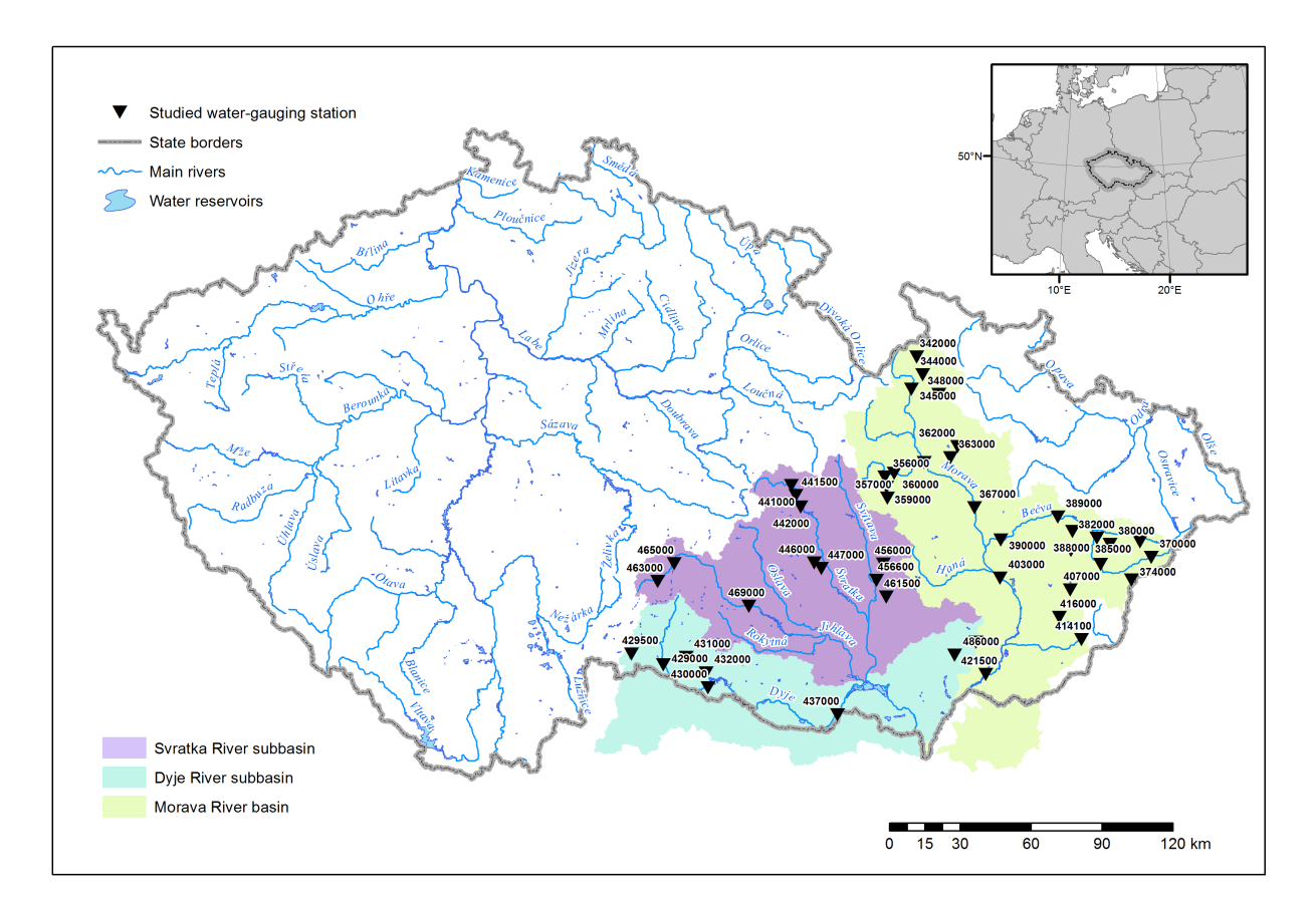
Fig. 1. Location of 46 selected water-gauging stations within the territory of Czechia
and their database numbers

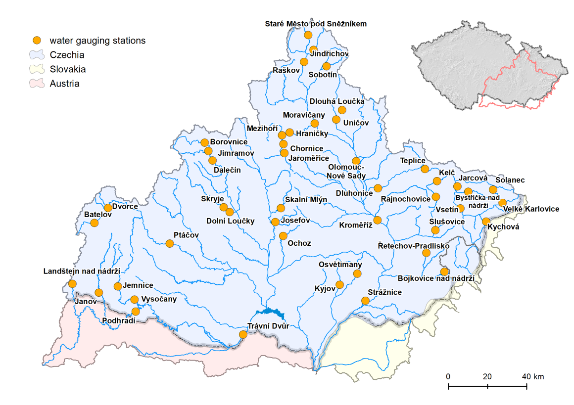
Fig. 2. A closer look at the study area of the Morava River basin and the 46 investigated
water-gauging stations together with their names

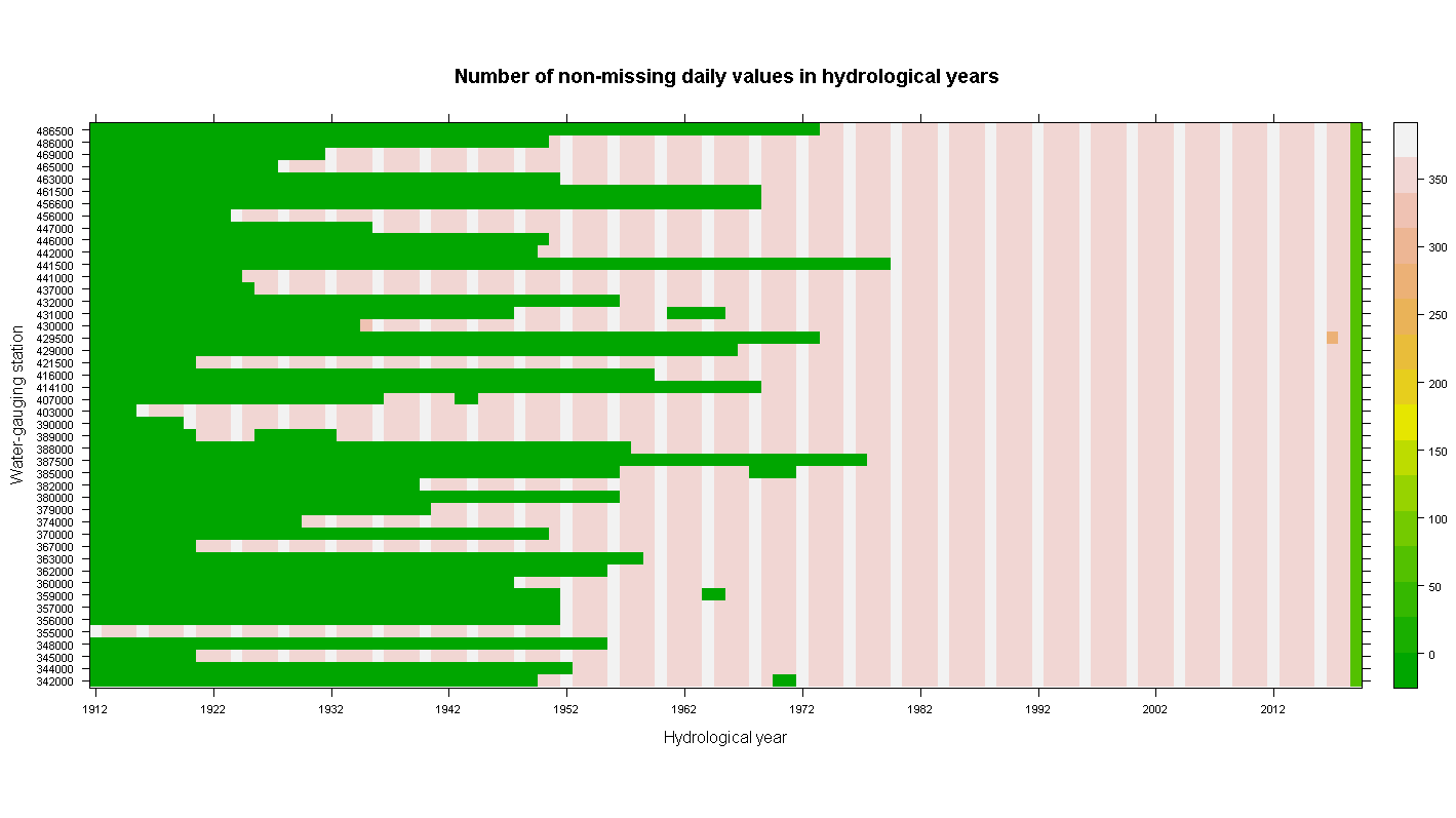
Fig. 3. Numbers of available mean daily discharge values at the 46 selected water-gauging stations in each hydrological year (previous November – actual October) of the period
from 1 November 1911 to 31 December 2018. The leap years naturally manifest themselves as lighter stripes. The green stripe at the end of the plot means that there were only the first two months available for the hydrological year 2019

Data imputation was performed by the function ‘na_kalman()’ which is part of the R package ‘imputeTS’ (see Moritz and Bartz-Beielstein, 2017, and the references therein). The structural model whose parameters were estimated by a maximum likelihood technique was then used for the estimation of a few missing QD values in 2017. Subsequent visual inspection of the time series plot (not shown) confirmed the validity of the model and the ‘na.contiguous()’ function could be then applied here as well. The other missing values were not estimated and addressing this issue was postponed to some of the future studies.

In the next step, two time periods were chosen:

1. the current Czech hydrological reference period 1981–2010 because we were curious about its representativeness, especially in relation to the recent dry episode having been experienced in Czechia, and
2. the longest period obtained by the R ‘na.contiguous()’ function that can be guessed from Fig. 3. Here, the beginnings of the QD series could naturally differ, but the ends were always 31 Decembers 2018.

Note, however, that for the purpose of analyzing streamflow drought-related indices, we set up a different start of the hydrological year. According to the recommendations in Fiala et al. (2010) and after the visual inspection of polar plots constructed separately for the reference period and the longest periods that show the typical timing of the occurrence of a low flow in the year (Fig. 4), we selected 1 April where, after spring snowmelt, the probability of the low-flow occurrence should be very low. The new hydrological years were then denoted according to the calendar years which shared the majority of the months. In order not to mix the natural processes that lead to the generation of droughts, the hydrological years were divided into the summer season (April–November) and to the winter season (December–March), similarly as in Fiala et al. (2010) or Ledvinka (2015a).

The division was made especially due to the planned analysis of low flows representing the minima for each season separately. Specifically, the series of following indices were derived from the QD series for each year of the longest periods and the reference period, respectively:

• Qmin7S representing the summer 7-day low flow and Qmin7W representing the winter 7day low flow,
• Qmin15S representing the summer 15-day low flow and Qmin15W representing the winter 15-day low flow,
• Qmin30S representing the summer 30-day low flow and Qmin30W representing the winter 30-day low flow.

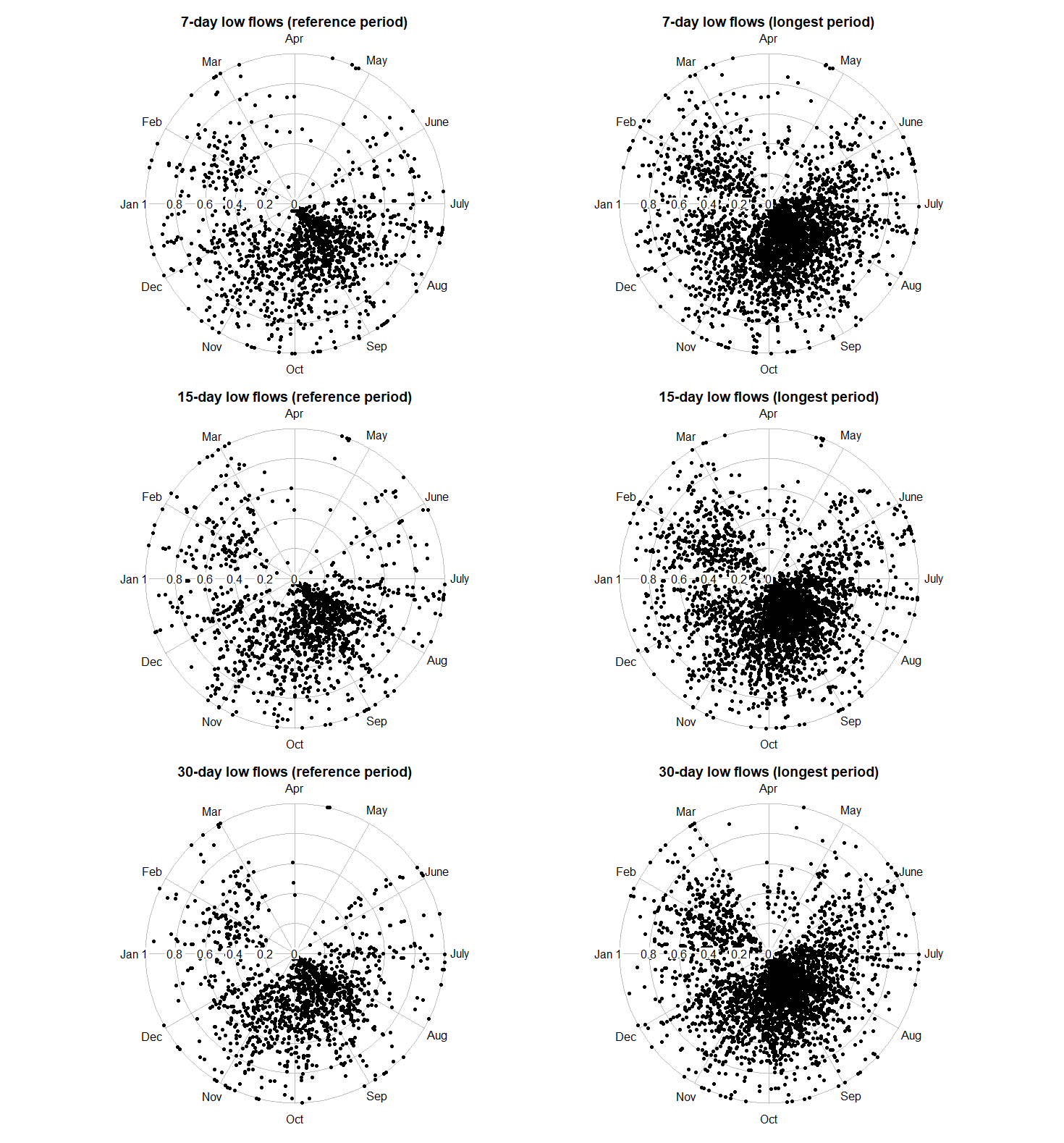
Fig. 4. Polar plots showing (by black dots) the timing of occurrences of standardized annual (either summer or winter minimum) 7-day, 15-day and 30-day low flows altogether
in each hydrological year of the reference period (left) and each possible hydrological year
of the longest periods (right) for all 46 investigated stations. The standardization was carried out for each station separately so that the maximum low flow over all years equals 1

When selecting and defining these indices, we were inspired by the work of Khaliq et al. (2008), and party by the work of Fiala et al. (2010) who analyzed only the seasonal 7-day low flows to which they added also the annual (mixed) 7-day low flows. First, the original QD series were filtered by respective moving averages (of window widths equal to 7, 15 and 30 days) and, then, their minima were extracted from the filtered series for each season. To accomplish this objective, we used the function ‘MAM()’ implemented in the ‘lfstat’ R package (Koffler et al., 2016) whose goal is to follow the methodology presented in the WMO manual (Gustard et al., 2008). However, the function had to be slightly modified so as to obtain also the Julian days corresponding to the first occurrences of the minima falling to the seasons, which allowed us to create Fig. 4. For the seasons where the filtered series were not complete (due to the use of centered moving averages), we did not extract any minima and, consequently, these seasons were not subjected to trend analyses. Further information about this type of indices coming from the QD series can, for instance, be found in Tallaksen and van Lanen (2004) or Tokarczyk (2013).

The second group of streamflow drought-related indices derived from the QD series used here were the so-called deficit volumes that, basically, represent the amount of water needed to be added to the stream so as to reach again a threshold that has not been equaled or exceeded for some time period. This time period is a typical accompanying variable of deficit volumes and is called the drought duration. The method through which the deficit volumes are calculated is called the threshold level method (TLM) which is an analogy of the peak-over-threshold (POT) method used for floods. Because, in the case of drought, one is interested in the opposite extreme, the TLM is sometimes called the pit-under-threshold (PUT) method (Gottschalk et al., 2013), or it has even other names in hydrology (Önöz and Bayazit, 2002). When looking for the missing amounts of water at our stations, we again employed the R package ‘lfstat’ (Koffler et al., 2016) and its function ‘find_droughts()’ where, in order to be as close as possible to reality and after gaining some experience in Czechia (e.g., Vlnas and Fiala, 2010), the 95th percentile of the flow duration curve (FDC) was set as the threshold that, moreover, was allowed to shift according to the months. This means that non-constant (seasonal) thresholds were set, even though Czech national standards consider only constant thresholds (COSMT, 2014). It is worth noting that only the thresholds defined for the reference period ensuring comparability of the results were used. Furthermore, since there may be some minor exceedances of the thresholds but, in fact, they should be part of longer drought periods, the so-called pooling techniques are very important here. For this purpose, we selected the sequent peak algorithm (SPA; see, e.g., Tallaksen et al., 1997; Tallaksen and van Lanen, 2004; Tokarczyk, 2013; Baran-Gurgul, 2018). Using the ‘summary()’ function applied to the object created by the function ‘find_droughts()’, we further left out the drought episodes with the duration less than 7 days and the deficit volumes with the magnitude lower than 0.5% of the maximum found for the station.

Finally, inspired by the paper of Hisdal et al. (2001), and setting zeroes for years with no drought episode, we got the time series of maximum and total deficit volumes and drought durations, both for the reference period and the longest possible periods for all the 46 water-gauging stations. Similar to the work of Ledvinka (2015b), we focused only on the summer season which, however, lasted until November. Namely, we obtained the series of the following indices (always for the 95th percentile of the FDC valid for the reference period):

• SSV95 representing the summer sums of deficit volumes,
• SSD95 representing the summer sums of drought durations,
• SMV95 representing the summer maxima of deficit volumes,
• SMD95 representing the summer maxima of drought durations that did not necessarily correspond to their deficit volume counterparts.

The last step was the trend analysis itself. Current studies indicate that there is a need to discriminate between STP and LTP before the application of a trend test because the original versions of the trend tests were designed for the data that are independent of each other, which, often, is not true in time series analysis in hydrology (Kundzewicz and Robson, 2000). This applies also to widely used nonparametric tests in hydrology such as the Mann–Kendall (MK) test that we wanted to employ. Therefore, we used the R package ‘HKprocess’ (Tyralis and Koutsoyiannis, 2011; Tyralis, 2016) and its function ‘MannKendallLTP()’ that, according to Hamed (2008), first checks whether the Hurst exponent, an important indicator of LTP, is significant. Depending on the results, we switched between the p-value accounting for LTP implemented in the R function ‘MannKendallLTP()’ or for STP (or white noise) in terms of the function ‘mmky1lag()’ which is part of the ‘modifiedmk’ R package (Patakamuri and O’Brien, 2019) and employs the MK test modification of Yue and Wang (2004). The direction of a significant trend (either at the 0.05 or 0.1 level of significance) was determined based on the Sen slope estimator (Sen, 1968) or the Kendall correlation coefficient measuring the dependence of a variable of interest on time (Kendall, 1970).

RESULTS AND DISCUSSION

A lot of results were obtained that were summarized in maps. The maps show that there are only very few significant changes in drought-related characteristics derived from the series of QD representing the Morava River basin, which corroborates the previous outcomes presented for the entire territory of Czechia (Fiala et al., 2010; Vlnas and Fiala, 2010; Ledvinka, 2015a, 2015b). It must be mentioned here that, apart from STP, we considered LTP as well, and exactly this might have caused the lowering of the number of expected trends (e.g., Cohn and Lins, 2005; Hamed, 2008). Notwithstanding, some trends can be observed that, moreover, cluster in typical regions. However, due to space limits, we decided to present only the most important maps here.

In the case of the longest periods the series SMD95 reveal very strong upward trends in the catchments of the rivers Branná (station Jindřichov), Fryšávka (station Jirmanov), Říčka (station Ochoz) and Juhyně (station Rajnochovice). The station Rajnochovice on the Juhyně shows an increase also in the series of SMV95 (see Fig. 5) and SSV95, which means that there must be groundwater resources drops as well. Otherwise, the groundwater would refill the surface waters on the northern slopes of the Hostýn Hills. Similar situation can be found in the catchment of the Fryšávka River which is a right-hand tributary of the Svratka River. The increasing trends at the Ochoz water-gauging station are interesting as well. Namely, the station is located below karstic springs. Here, one can observe an increasing trend in all the variables connected with the deficit volumes. From the perspective of the reference period 1981–2010, the station Bystřička nad nádrží (Bystřice River) unveils increasing trends in both deficit volumes and their durations, no matter when it comes to the summer maxima or sums. This can be valuable knowledge for water managers who manipulate the outflow from the reservoir Bystřička, as this situation may be repeated in the future.

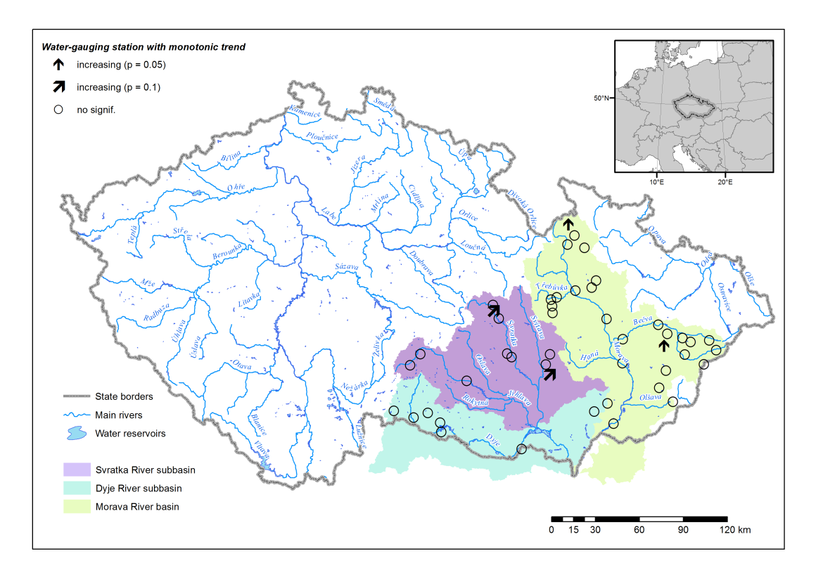
Fig. 5. Trends in the series of summer maxima of deficit volume for the longest periods

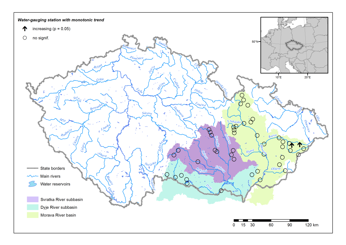
Fig. 6. Trends in the series of summer sums of drought duration for the reference period

After the analyses of summer (April–November) minima, and taking into account the longest periods, trends in the series of Qmin7S must be stressed that point to the decreases in water levels of streams draining the karst (see stations Ochoz and Josefov in Fig. 7). The spatial pattern of deficit volumes is somewhat inherited here as well. Namely, the station Rajnochovice on the Juhyně can be mentioned as an example. There are also subbasins of the Morava River basin where the same directions of trends occur regardless of the length of the smoothing window applied to the series of QD. The indices Qmin7S, Qmin15S and Qmin30S reveal substantial decreases at stations Sobotín (Merta River), Dlouhá Loučka (Loučka River), above-mentioned Ochoz, Josefov and Rajnochovice, Solanec (Hutisko Brook), and Bojkovice nad nádrží (Kolelač Brook). Regarding the reference period and the summer season, the Bystřička nad nádrží water-gauging station should be highlighted where the shift to the lower values of filtered QD series has been recorded for all the three indices corresponding to discharge minima. It seems that there is a good consistency between deficit volumes and minima, and, without a doubt, water manages should be aware of this behavior of the Bystřice River above the water reservoir. When looking only at wider smoothing windows, namely at the series of Qmin15S and Qmin30S (Fig. 8), the station Řetechov-Pradlisko indicates drops in the water levels of the Ludkovice Brook.

On the contrary, the winter season (December–March) shows also the opposite directions of the development of discharge minima. Nevertheless, for the longest periods, it is true that we have observed prevailing downward trends, namely for the station Josefov (Křtiny Brook) where this pattern is supported by all the indices Qmin7W, Qmin15W and Qmin30W. However, when looking at the minima represented by Qmin7W (Fig. 9) and Qmin15W, upward trends are apparent at the Skryje water gauging station (Bobrůvka River), indicating that the winter seasons may be characterized rather by rising discharge here, which is especially contradictory to the situation in summer 2018 with, historically, the lowest discharge values in this catchment. Of course, the very dry period 2014–2018 can be visible only using the longest periods analyzed here and the information what happens before the summer low flows occur is more than valuable. The phenomenon of larger discharge minima in winters that do not correspond to the tendencies occurring in summers may be attributed to the changes relating to the snow cover, likely triggered by a warming climate (Jenicek et al., 2016). The rising low flows at the Kychová station (i.e. the smallest catchment of the Kychová River with relatively long QD series; see Fig. 9) should definitely be studied from this point of view as well. Having merely the data from the reference period would force us to conclude that, at a number of water-gauging stations in the Morava River basin, rather mitigation of winter low flows occurred until 2010. For all the indices Qmin7W, Qmin15W and Qmin30W, it happened in the Upper Morava River basin and in the Lower Bečva River basin – stations Staré Město pod Sněžníkem and Dlouhá Loučka for the Morava and Teplice and Dluhonice for the Bečva, respectively. Nevertheless, most increasing trends can be found for the case corresponding to the monthly width of the smoothing windows (i.e., for Qmin30W; see Fig. 10).

Fig. 7. Trends in the series of summer 7-day low flows for the longest periods

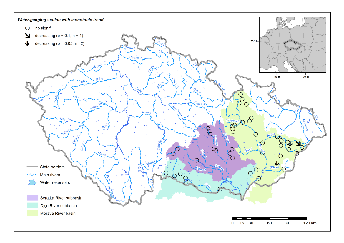
Fig. 8. Trends in the series of summer 30-day low flows for the reference period

At first glance, a compensation process occurring in winters might come across one’s mind. However, before suggesting this, it would be necessary to know what happens now with snow in winters. During higher air temperatures, snow and ice may melt earlier than in the past, and the ratio of liquid precipitation to water stored in snow and ice probably rises. This all may cause the precipitation water to join the runoff much faster in current winters, which, on the other hand, does not necessarily mean that the overall water balance changes as well. Rather, the seasonal course changes in accordance with the behavior of snow cover, which may have crucial effects on the occurrence of summer low flows (Jenicek and Ledvinka, 2019). Therefore, the pattern of increasing winter low flows (northern slopes of the Hostýn Hills, upper basins of the Jihlava River, the Morava River, the Svratka River, and eastern slopes of the Drahany Highlands), should be considered with caution.

Fig. 9. Trends in the series of winter 7-day low flows for the longest periods

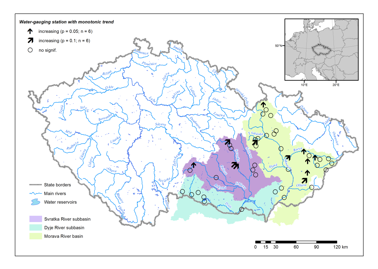
Fig. 10. Trends in the series of winter 30-day low flows for the reference period

CONCLUSIONS AND RECOMMENDATIONS

In this study, trends in streamflow drought-related indices were sought using the hypothesis tests that account for STP or LTP, namely the modifications of the MK test that have been developed in hydrology. The basin of the Morava River, and specifically the series of QD from 46 selected water-gauging stations were investigated, either for the case of the Czech reference hydrological period or the longest periods allowed by the lengths of the QD series. The analyses were done separately for the summer seasons (April–November) and winter seasons (December–March). The results show that, although the basin currently suffers from a long-lasting drought episode, there are almost no significant trends in the indices including the 7-, 15- and 30-day low flows or the deficit volumes and the drought durations. If some, one can observe rather increases in summer deficit volumes, which corresponds to the decreases in summer low flows, especially in the karst areas. On the other hand, winter low flows indicate that the Morava River basins experiences some changes in snow cover, likely due to a warming climate. It is apparent that, now, the snow cover melts earlier (or the ratio of liquid precipitation is getting higher) in winters, which causes the winter low flows to rise at some places. However, we assume that these rising low flows do not compensate the water deficits occurring in summers. Rather, they indicate the shifts in seasonal course that may have an adverse influence on the summer discharge (Jenicek and Ledvinka, 2019).

Regarding the reference period, some decreases in water resources above the Bystřička water reservoir were detected that water managers should take into account in the future. However, we are aware of the fact that a 30-year period is relatively short for the estimation of the Hurst exponent, an important characteristic indicating LTP (Montanari, 2003), and the results of the subsequent trend analyses may be somewhat biased. Therefore, we recommend that the longest periods should be analyses in the future. Looking at the lengths of the available discharge series (Fig. 3), one should also pay more attention to the missing values that could be filled in based on a rigorous imputation technique (e.g., Moritz and Bartz-Beielstein, 2017). One could also look at the frequency of the occurrence of dry episodes within each year in a similar way to Hisdal et al. (2001). Last but not least, we suggest studying physical-geographical characteristics of the catchments (such as those in Table A.1) so as to better understand the clustering of detected trends. Other types of changes in the series of the indices (i.e., different from gradual or monotonic ones) should be investigated as well.

ACKNOWLEDGEMENTS

The authors would like to thank especially to the team of Petr Šercl from the Surface Water Department of the Czech Hydrometeorological institute who carried out the investigation of the Czech water-gauging stations and highlighted those suitable for low-flows studies, which substantially helped us select the 46 stations for the Morava River basin.

APPENDIX

Table A.1. Basic morphometric characteristics of 46 selected subbasins of the Morava River basin delineated by the water-gauging stations for which the streamflow drought-related indices were

computed

Note: Hyphens indicate that, currently, the characteristics could not be computed easily because parts of the subbasins lie in the territory of Austria for which we did not have any digital elevation models at hand. Basin shape ranges from (stretched basins) to 1 (circular-shaped basins).

REFERENCES 

Baran-Gurgul K. 2018. A comparison of three parameter estimation methods of the gamma distribution of annual maximum low flow duration and deficit in the Upper Vistula catchment (Poland). ITM Web of Conferences, 23: 00001. https://doi.org/10.1051/itmconf/20182300001.

CHMI. 2018a. Suché období 2014-2017: vyhodnocení, dopady a opatření [Dry Period 2014–2017: Evaluation, Impacts and Measures]. Czech Hydrometeorological Institute: Praha.

CHMI. 2018b. Vyhodnocení sucha na území kraje Vysočina za období 2015-2018 [Drought Evaluation in the Vysočina Region in 2015 – September 2018]. Czech Hydrometeorological Institute: Brno.

CHMI. 2019. Sucho 2014-2018: sborník abstraktů [Drought 2014–2018: Book of Abstracts]. Czech Hydrometeorological Institute: Praha.

Cohn TA, Lins HF. 2005. Nature’s style: naturally trendy. Geophysical Research Letters, 32(23): L23402. https://doi.org/10.1029/2005GL024476.

COSMT. 2014. Hydrologické údaje povrchových vod [Hydrological Data on Surface Water]. Czech Office for Standards, Metrology and Testing: Praha.

Daňhelka J, Bercha Š, Boháč M, Crhová L, Čekal R, Černá L, Elleder L, Fiala R, Chuchma F, Kohut M, Kourková H, Kubát J, Kukla P, Kulhavá R, Možný M, Reitschläger JD, Řičicová P, Sandev M, Skřivánková P, Šercl P, Štěpánek P, Valeriánová A, Vlnas R, Vrabec M, Vráblík M, Zahradníček P, Zrzavecký M. 2015. Vyhodnocení sucha na území České republiky v roce 2015 [An Assessment of the Drought in the Territory of the Czech Republic in 2015]. Czech Hydrometeorological Institute: Praha.

Daňhelka J, Kubát J (eds). 2019. Vyhodnocení sucha na území České republiky v roce 2018 [An Assessment of the Drought in the Territory of the Czech Republic in 2018]. Czech Hydrometeorological Institute: Praha.

Fiala T, Ouarda TBMJ, Hladný J. 2010. Evolution of low flows in the Czech Republic. Journal of Hydrology, 393(3–4): 206–218. https://doi.org/10.1016/j.jhydrol.2010.08.018.

Gottschalk L, Yu K, Leblois E, Xiong L. 2013. Statistics of low flow: Theoretical derivation of the distribution of minimum streamflow series. Journal of Hydrology, 481: 204–219. https://doi.org/10.1016/j.jhydrol.2012.12.047.

Gustard A, Demuth S, Parker S (eds). 2008. Manual on Low-Flow Estimation and Prediction. WMO: Geneva.

Hamed KH. 2008. Trend detection in hydrologic data: the Mann–Kendall trend test under the scaling hypothesis. Journal of Hydrology, 349(3–4): 350–363. https://doi.org/10.1016/j.jhydrol.2007.11.009.

Hisdal H, Stahl K, Tallaksen LM, Demuth S. 2001. Have streamflow droughts in Europe become more severe or frequent? International Journal of Climatology, 21(3): 317–333. https://doi.org/10.1002/joc.619.

Jenicek M, Ledvinka O. 2019. Modelling the impact of changes in seasonal snowpack on annual runoff and summer low flows. Geophysical Research Abstracts, 21: Article no. EGU2019-9879.

Jenicek M, Seibert J, Zappa M, Staudinger M, Jonas T. 2016. Importance of maximum snow accumulation for summer low flows in humid catchments. Hydrology and Earth System Sciences, 20(2): 859–874.

https://doi.org/10.5194/hess-20-859-2016.

Kendall MG. 1970. Rank Correlation Methods. Griffin: London.

Khaliq MN, Ouarda TBMJ, Gachon P, Sushama L. 2008. Temporal evolution of low-flow regimes in Canadian rivers. Water Resources Research, 44(8): W08436. https://doi.org/10.1029/2007WR006132.

Koffler D, Gauster T, Laaha G. 2016. lfstat: Calculation of Low Flow Statistics for Daily Stream Flow Data. R package version 0.9.4. https://CRAN.R-project.org/package=lfstat.

Kundzewicz ZW, Robson A (eds). 2000. World Climate Programme - Water. Detecting Trend and Other Changes in Hydrological Data. WMO: Geneva.

Ledvinka O. 2015a. Evolution of low flows in Czechia revisited. Proceedings of the International Association of Hydrological Sciences, 369: 87–95. https://doi.org/10.5194/piahs-369-87-2015.

Ledvinka O. 2015b. Trends in summer hydrological droughts in Czechia with respect to the scaling hypothesis. Water-Food-Energy River and Society in the Tropics. paper presented at the 10th Alexander von Humboldt International Conference. Copernicus Publications: Addis Ababa, Ethiopia, AvH10-19.

Montanari A. 2003. Long-range dependence in hydrology. In: Doukhan P, Oppenheim G and Taqqu MS (eds) Theory and Applications of Long-Range Dependence. Birkhäuser: Boston, Massachusetts, 461–472.

Moritz S, Bartz-Beielstein T. 2017. imputeTS: Time series missing value imputation in R. The R Journal, 9(1): 207–218. https://doi.org/10.32614/RJ-2017-009.

Önöz B, Bayazit M. 2002. Troughs under threshold modeling of minimum flows in perennial streams. Journal of Hydrology, 258(1–4): 187–197. https://doi.org/10.1016/S0022-1694(01)00562-5. Patakamuri SK, O’Brien N. 2019. modifiedmk: Modified Versions of Mann Kendall and Spearman’s Rho Trend Tests. R package version 1.4.0. https://CRAN.R-project.org/package=modifiedmk.

Sen PK. 1968. Estimates of the regression coefficient based on Kendall’s tau. Journal of the American Statistical Association, 63(324): 1379–1389. https://doi.org/10.2307/2285891.

Šercl P, Kukla P, Daňhelka J, Kurka D. 2016. Reprezentativnost profilů vodoměrných stanic pro měření a vyhodnocení minimálních průtoků [The representativeness of gauging stations for the measurement and evaluation of low flows]. Hydrological Yearbook of the Czech Republic 2015. Czech Hydrometeorological Institute: Praha, 178–181.

Šercl P, Kukla P, Pecha M, Němec L, Černá L. 2019. Zhodnocení vývoje hydrologické situace v období 20142018 [An assessment of the development of hydrological situation in the period 2014–2018]. Hydrological Yearbook of the Czech Republic 2018. Czech Hydrometeorological Institute: Praha, (in preparation).

Tallaksen LM, Madsen H, Clausen B. 1997. On the definition and modelling of streamflow drought duration and deficit volume. Hydrological Sciences Journal, 42(1): 15–33. https://doi.org/10.1080/02626669709492003.

Tallaksen LM, van Lanen HAJ (eds). 2004. Hydrological Drought: Processes and Estimation Methods for Streamflow and Groundwater. Elsevier: Amsterdam; Boston.

Tokarczyk T. 2013. Classification of low flow and hydrological drought for a river basin. Acta Geophysica, 61(2): 404–421. https://doi.org/10.2478/s11600-012-0082-0.

Tyralis H. 2016. HKprocess: Hurst-Kolmogorov Process. R package version 0.0-2. https://CRAN.Rproject.org/package=HKprocess.

Tyralis H, Koutsoyiannis D. 2011. Simultaneous estimation of the parameters of the Hurst–Kolmogorov stochastic process. Stochastic Environmental Research and Risk Assessment, 25(1): 21–33. https://doi.org/10.1007/s00477-010-0408-x.

Vizina A, Hanel M, Trnka M, Daňhelka J, Gregorieová I, Pavlík P, Heřmanovský M. 2018. HAMR: online systém pro zvládání sucha - operativní řízení během suché epizody [HAMR: online drought management system - operational management during a dry episode]. Water Management Technical and Economical Information Journal, 60(5): 22–28.

Vlnas R, Fiala T. 2010. Spatial and temporal variability of hydrological drought in the Czech Republic. SGEM2010 Conference Proceedings. paper presented at the 10th International Multidisciplinary Scientific Geoconference and EXPO - Modern Management of Mine Producing, Geology and Environmental Protection, SGEM 2010. International Multidisciplinary Scientific Geoconference: Varna, Bulgaria, 59–66.

Whitfield PH, Burn DH, Hannaford J, Higgins H, Hodgkins GA, Marsh T, Looser U. 2012. Reference hydrologic networks I. The status and potential future directions of national reference hydrologic networks for detecting trends. Hydrological Sciences Journal, 57(8): 1562–1579. https://doi.org/10.1080/02626667.2012.728706.

Yue S, Wang C. 2004. The Mann-Kendall test modified by effective sample size to detect trend in serially correlated hydrological series. Water Resources Management, 18(3): 201–218. https://doi.org/10.1023/B:WARM.0000043140.61082.60.

Back to CONTENTS