ASSESSMENT HARMONIZATION PROBLEMS
OF THE LONG RETURN PERIOD FLOODS ON THE DANUBE RIVER

Pavla Pekárová¹, Pavol Miklánek¹, Veronika Bačová Mitková¹, Marcel Garaj¹, Ján Pekár2

1Institute of Hydrology SAS, Dúbravskú cesta 9, 841 04 Bratislava, Slovakia

2 Comenius University in Bratislava, Faculty of Mathematics, Physics, and Informatics, Bratislava, Slovakia

Corresponding author: Pavla Pekárová, Institute of Hydrology SAS, Dúbravskú cesta 9, 841 04 Bratislava, Slovakia,

Pekarova@uh.savba.sk

ABSTRACT

One of the basic problems of the flood hydrology was (and still is) the solution of the relationship between peak discharges of the flood waves and probability of their return period. The assessment of the design values along the Danube channel is more complicated due to application of different estimation methods of design values in particular countries downstream the Danube. Therefore, it is necessary to commence the harmonization of the flood design values assessment methods. All methods of estimating floods with a very long return period are associated with great uncertainties. Determining of the specific value of the 500- or 1000-year floods for engineering practice is extremely complex. Nowadays hydrologists are required to determine not only the specific design value of the flood, but it is also necessary to specify confidence intervals in which the flow of a given 100-, 500-, or 1000-year flood may occur with probability, for example, 90 %.

The assessment of the design values Qmax can be done by several methods. In this study we have applied the statistical methods based on the assessment of the distribution function of measured time series of the maximum annual discharge. In order to apply regionalization methods for the estimation of the distribution function in this study we used only one distribution - the Pearson Type III distribution with logarithmic transformation of the data (log Pearson Type III distribution - LP3 distribution). To estimate regional skew coefficient for the Danube River we use 20 Qmax measured time series from water gauges along the Danube River from Germany to Ukraine. We firstly analyzed the occurrence of historic floods in several stations along the Danube River. Then we search relationship between the parameter of skewness of the log Pearson type III distribution function and runoff depth, altitude, or basin area in all 20 water gauge. Skewness coefficients of the LP3 distribution in the stations along the Danube River vary between –0.4 and 0.86.

Keywords: floods, design values, Danube River, LP3 distribution, regionalization.

INTRODUCTION

Under the present and foreseeable human activities to a sustainable development of the industry, agriculture, energy and water supply the demands of the hydrological synthetic characteristics of the flow regime are continuously increasing (Stănescu, 2004). One of the basic problems of the flood hydrology was (and still is) the solution of the relationship between peak discharges of the flood waves and probability of their return period. Importance of extrapolation derived from these variables (so called frequency curve) is especially necessary for proposal of water management and flood control plans. Directive 2007/60/ EC of the European Parliament of 23 October 2007 concerning the assessment and management of flood risks requires member States to draw up flood hazard maps of floods with very long return periods T (500 to 1000 years).

The main steps of the statistical processing are the following:

1) Selection of the time series of the maximum discharges:

a) the maximum annual discharges Qmax, or

b) the maximum discharges exceeding a certain threshold value.

A big problem of the hydrological regionalization refers to the manner in which the transfer of data to the ungauged basins or to deficient data sites is carried out. There are two main procedures to perform this transfer: the first one consists in finding out some relationships aiming to the spatial interpolation of the principal statistics of the probability curves. The second procedure tries to eliminate the shortcoming of the first one. This consists in finding out several statistical distribution curves of standardized annual maximum discharge. Standardization is achieved by dividing the maximum annual discharges by their average magnitude Q. These standardized (or dimensionless) curves are often called growth curves (Stănescu, 2004).

All methods of estimating floods with a very long return period are associated with great uncertainties. Determining the specific value of a 500- or 1000-year flood for engineering practice is extremely complex. Nowadays hydrologists are required to determine not only the specific design value of the flood, but it is also necessary to specify confidence intervals in which the flow of a given 100-, 500-, or 1000-year flood may occur with probability, for example, 90 %. Estimation of the uncertainty at the design discharges was investigated for example by Szolgay et al. (2003), Merz et al. (2004), or Rogger et al. (2012). It is generally known, that the extrapolation of the data is very sensitive not only to the length of the data series, but also to the inclusion of the historic extremes to data series. The correct estimations of potential culminations of floods require the inclusion of the longest data series of observations, as well as the inclusion of historic pre-instrumental data to statistically analysed data series (Lauda et al., 1908; Kresser, 1957; Merz and Blöschl 2008a,b; Elleder 2010; Gaal et al., 2010; Elleder et al., 2013; Kjeldsen et al., 2014). Brazdil et al. (2006) studied historic hydrological materials in order to estimate floods threat in Europe.

Except the mentioned factors the estimation of the T-year discharges is finally influenced by used type of the theoretical probability distribution function. The choice of the type of the theoretical probability distribution function should relatively accurately represent uncertainty and variability of the hydrological problem. Application and choice of a particular probability distribution function, method of the parameter estimation as well as choice of the analyzed period depend on the calculation method commonly used in a particular country. For large international basins such as the Danube River basin, it is necessary to synchronize the methodology and to prepare common procedures for determining flood hazard. Investigation of the history of extreme flood event frequency, severity and duration provides a greater understanding of the region’s extreme event characteristics and the probability of recurrence at various levels of severity. This type of information is beneficial in the development of extreme response and mitigation strategies and preparedness plans.

The aim of the paper is to propose unified methodology to estimate the design values of flood discharges in stations along the Danube River. Here we present the results of the estimation of the Qmax discharge series distribution function using log Pearson Type III distribution (LP3) with inclusion of the historical floods into data series. We focused on estimation of the relationship between the skew coefficient of the log Pearson type III distribution function and runoff depth on the base of data from 20 water gauges along the Danube River.

METHODS

As it was mentioned, for the estimation of the Qmax discharge series distribution function we used the log Pearson Type III distribution. The Pearson Type III, or Gamma, distribution is used to calculate the frequency of maxima events when the distribution of all events (both big and small) is log-normally distributed. In hydrologic applications, the log-normal distribution has been found to reasonably describe such variables as the depth of precipitation of individual storms and annual peak discharges Griffis and Stendinger (2007 and 2009). Today, the application of LP3 distribution to quantify the recurrence interval of large peak annual discharges is recommended by the U.S. Interagency Advisory Committee on Water Data ("Guidelines for Determining Flood Flow Frequency", Bulletin 17B of the Hydrology Committee, U.S. Geological Survey, Reston, VA). It is the default distribution used by the U.S. Geological Survey for flood studies (Koutsoyiannis, 2008). Pilon and Adamowski (1993) developed the Log Likelihood function of LP3 and estimated its parameters. Cheng et al. (2007) presented a frequency factor-based method in hydrological frequency analysis for random generation of five distributions (normal, lognormal, extreme value type 1, Pearson Type III and log-Pearson Type III). He used LP3 distribution in flood frequency analysis too. Some authors (Stedinger and Griffis 2008) preferred the Generalized Extreme Value distribution (GEV). Comparison of several types of distributions (GEV, LP3 and Gumbel) for estimating T-year discharges presented Millington et al. (2011). Authors did not prefer any distribution as better and they suggested other researches in this problem.

Stănescu (2004) used for the extrapolation of the regional curves in Danube Basin the Pearson III curves. Using one type of distribution also allows to estimate the value of the T-year maximum discharges in parts of the river without observations, only on the basis of long-term average of maximum annual discharge and distribution parameters from the neighboring gauging stations.

In this study, to estimate the distribution parameters, the method described in Bulletin17B was used. Bulletin 17B was issued in USA in 1981, and re-issued with minor corrections in 1982 in the Centre for Research in Water Resources of the University of Texas at Austin (IACWD, 1982). Bulletin 17B provided revised procedures for weighting station skew values with results from a generalized skew study, detecting and treating outliers, making two station comparisons, and computing confidence limits about a frequency curve. Bulletin 17B is based on Bulletins 15, 17, 17A (http://acwi.gov/hydrology/ Frequency/minutes/index.html). (Design flood estimation procedures in the United States have traditionally focused on two primary methods: frequency analysis of peak flows for floodplain management and levee design; and deterministic – Probable Maximum Flood estimates – for design of dams and nuclear facilities.)

The log-Pearson Type III distribution is a three-parameter Gamma distribution with a logarithmic transform of the variable. It is widely used for flood analyses because the data quite frequently fit the assumed annual maximum discharge series. The probability density function of the Pearson Type III distribution is of the form:

(1)

with , where 𝜏, 𝛼, 𝛽 are parameters:
𝜏 – is the location parameter;
𝛼 – is the shape parameter;
𝛽 – is the scale parameter;
Γ(𝛼) is the Gamma function given by:

.� (2)

Random variable X follows log-Pearson type III distribution if random variable 𝑌 = 𝑙𝑛𝑋 or
𝑌 = 𝑙𝑜𝑔𝑋 follows the Pearson type III distribution. Log-normal distribution is a special case of the log-Pearson type III distribution when skew coefficient of logarithmic data is equal to zero.
The distribution is fit by computing the base 10 logarithms of the discharge, Q, at a selected exceedance probability, p, using the following equation:

� (3)

where:
is the mean,
S is the standard deviation, and
K is a factor of the skew coefficient at selected exceedance probability.
The formulas for these parameters are provided below.

Mean� .� (4)

Standard Deviation� .� (5)
Skew Coefficient � . (6)

Probability estimates are made using plotting positions. A basic plotting position formula for symmetrical distributions is (Stedinger et al., 1993, p. 18.24)

,� (7)

where 𝑝𝑖 is the exceedance probability of flood observations 𝑄𝑖 ranked from largest (i = 1) to
smallest (i = n), and a is a plotting position parameter, (0 ≤ 𝑎 ≤ 0.5).
The method of moments uses the logarithms of flood flows to estimate the distribution parameters. The first three sample moments are used to estimate the LP3 parameters. These include the mean (𝜇̂), standard deviation (𝜎̂), and skewness coefficient (𝛾̂).
In the case where only systematic data are available, with no historical information, the mean, standard deviation and skewness coefficient of station data may be computed using the following equations:
� (8)

� (9)

,� (10)

where n is the number of flood observations and (ˆ) represents a sample estimate.

Historical floods

Historical flood peaks reflect the frequency of large floods and thus should be incorporated into flood frequency analysis. They can also be used to judge the adequacy of estimated flood frequency relationships. For this latter purpose, appropriate plotting positions or estimates of the average exceedance probabilities associated with the historical peaks and the remainder of the data are desired. Hirsch and Stedinger (1987) and Hirsch (1987) provide an algorithm for assigning plotting positions to censored data, such as historical floods.

Weighted Skew Coefficient

There is relatively large uncertainty in the site sample skewness coefficient (third moment) because it is sensitive to extreme events in modest length records (Griffis and Stedinger, 2007a). The station skew coefficient and regional skew coefficient can be combined to form a better estimate of skew for a given watershed. Under the assumption that the regional skew coefficient is unbiased and independent of the station skew, the mean-square errors (MSEs) of the station skew and the regional skew can be used to estimate a weighted skew coefficient.

If the regional and station skews differ by more than 0.5, a careful examination of the data and the flood-producing characteristics of the watershed should be made. Possibly greater weight may be given to the station skew, depending on record length, the largest floods within the gauging record and watershed, and watershed characteristics. Large deviations between the regional skew and station skew may indicate that the flood frequency characteristics of the watershed of interest are different from those used to develop the regional skew estimate. It is thought that station skew is a function of rainfall skew, channel storage, and basin storage. There is considerable variability of response among different basins with similar observable characteristics, in addition to the random sampling variability in estimating skew from a short record. It is considered reasonable to give greater weight to the station skew, after due consideration of the data and flood-producing characteristics of the basin.

Uniform technique for determining flood discharge frequencies

We added the historic floods to the measured series of Qmax, and we recalculated the parameters of the distribution curves for individual stations having included the historic floods.

The Frequency curve spreadsheet version 3.06 (Dan Moor, August 2014) was used to estimate the parameters of distribution functions and to calculate the design values.

Qmax series conditions

Among the basic assumptions for application of the frequency analysis of the maximum annual discharge belong the following conditions:

Maximum annual discharges must be independent and stochastic;
Processes influencing the runoff process are stationary with respect to time (homogeneity of the series);
Statistical characteristics of the measured data series (series of maximum annual discharge) represent the past, presence and future, as well.

DANUBE BASIN DESCRIPTION

The Danube River with a total length of 2857 km and a long term daily mean discharge of about 6500 m3s-1 is listed as the second biggest river in Europe. In terms of length it is listed as the 21st biggest river in the world, in terms of drainage area it ranks as 25th with a drainage area of 817,000 km2. The Danube basin extends from the central Europe to the Black Sea. The extreme points of the basin are 8º 09ʹ and 29º 45ʹ of the Eastern longitude, and 42º 05ʹ and 50º 15ʹ of the Northern latitude (Stancik & Jovanovic, 1988). More recent estimation of the Danube basin area was done by the International Commission on Protection of the Danube River (ICPDR, 2005) which calculated the areas using GIS on the basis of the Danube River Basin District overview map. According to the estimation of the ICPDR the total area of the Danube river basin is 801,463 km2 (Fig. 2).

Nineteen countries share the Danube basin, though two thirds of the catchment lie within five countries (Romania, Hungary, Serbia, Austria and Germany). The Danube River originates in the Schwarzwald (Black Forest) mountains in Bavaria in Germany. It has its sources outside the Alps in an old mountainous massif. The Breg, which is the longer of the two streams that form the river Danube, begins at only 1,078 m above sea level, 100 m from the European Water Divide. In the case of the Danube River Basin, its landscape geomorphology is characterized by a diversity of morphological patterns and the river channel itself can be divided into 6 sections (Fig. 1) according to the river slope (Lászlóffy, 1965). The main tributaries of the Danube River are shown in Fig. 2.

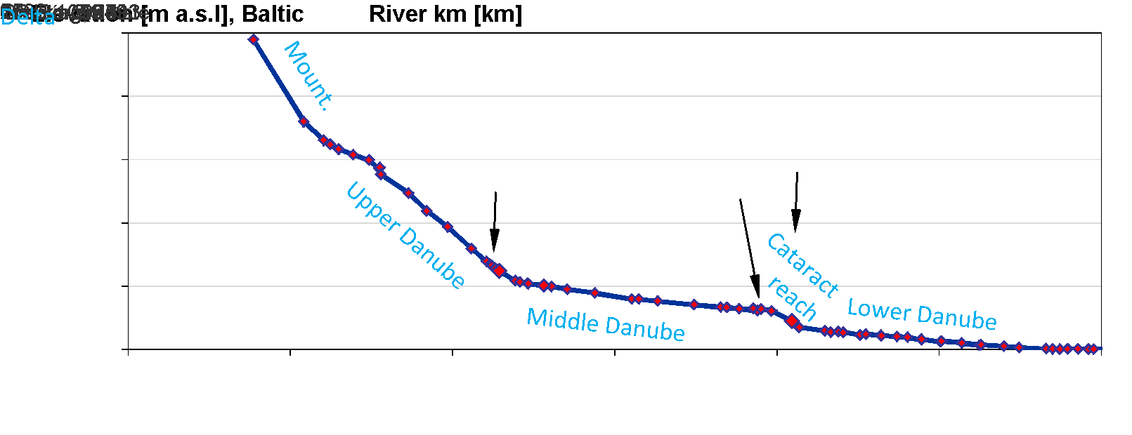
Fig. 1. The Danube River sections

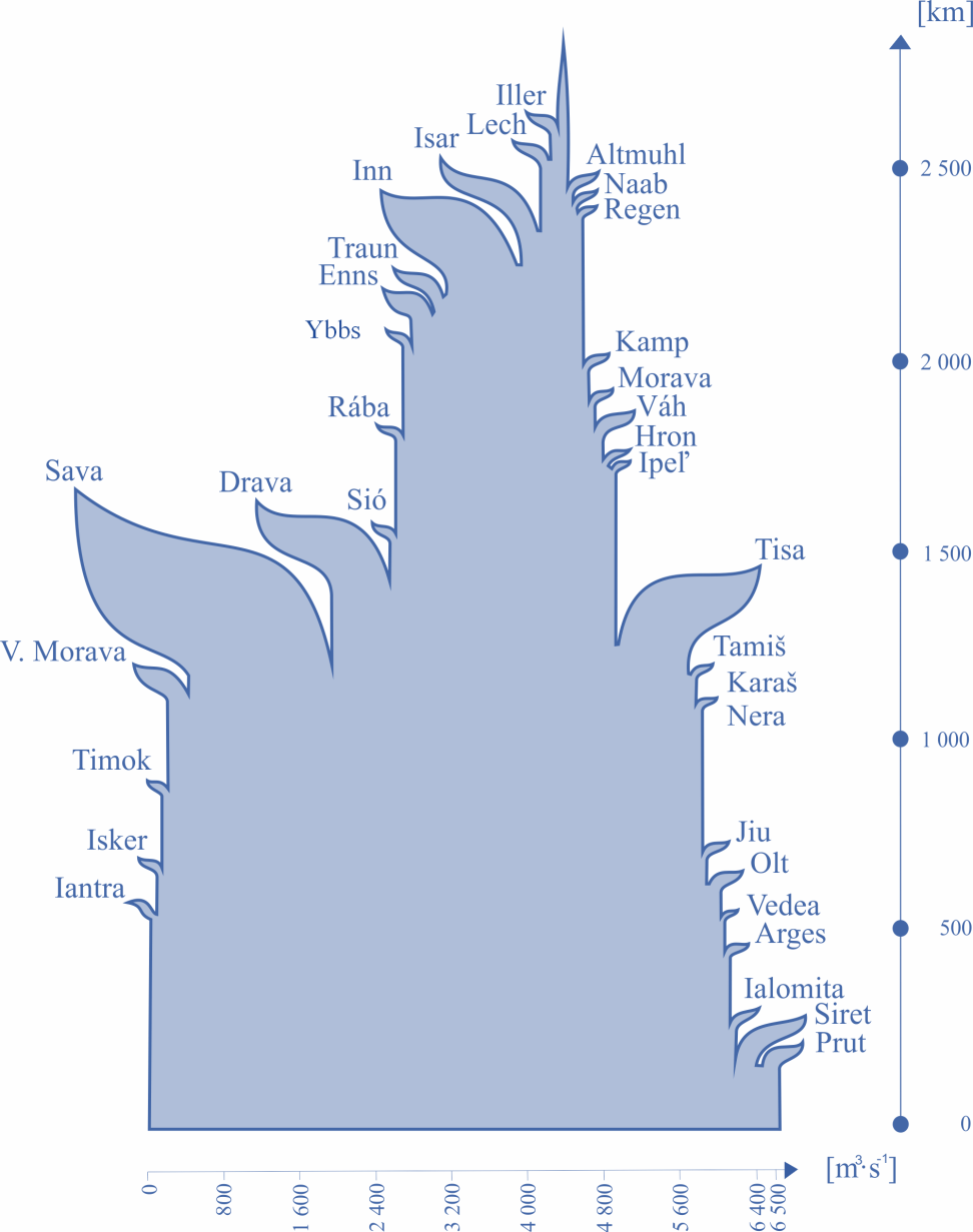
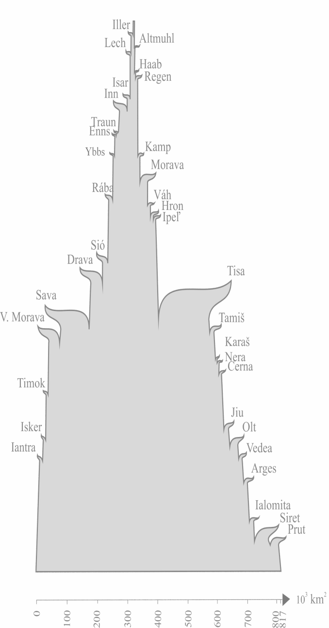
$K:\Pavla\clanky\clanky19\Dunajska konf\text Omax Danube\Dunaj_pritoky_modra_s_obrysom_ciernej_1.PNG$ $K:\Pavla\clanky\clanky19\Dunajska konf\text Omax Danube\velkostpovodia3.PNG$

Fig. 2. The Danube and its tributaries, discharge, and area scheme

DATA DESCRIPTION

Flooding is the most common natural disaster in the Danube River basin and, in terms of economic damage, the costliest one. In case of the Danube River from Achleiten downstream the duration of the floods is longer than one day. Therefore, the flood peak discharges differ very rarely from the mean daily discharges of the day when the flood peak did occur. In Fig. 3 there are presented examples of the maximum annual discharges in the upper (Hofkirchen gauge), in the middle (Bratislava gauge) and lower Danube (Orsova/Turnu Severin gauge, and Reni gauge) from 95 to 170 years.

It is interesting that similar maximum discharges as in the last period did occur also at the end of the 19th century in both stations. Very significant floods occurred on the lower Danube in 2006 (peak discharge 15,900 m3s-1 at Ceatal Izmail), and on the upper Danube in 2013 (peak discharge 10,640 m3s-1 at Bratislava and 9,460 m3s-1 at Budapest).

To estimate regional skew coefficient of the LP3 distribution for Danube River we use 20 Qmax measured time series from water gauges along the Danube River from Germany to Ukraine (Fig. 4). Basic statistical characteristics of the stations are presented in Table 1.

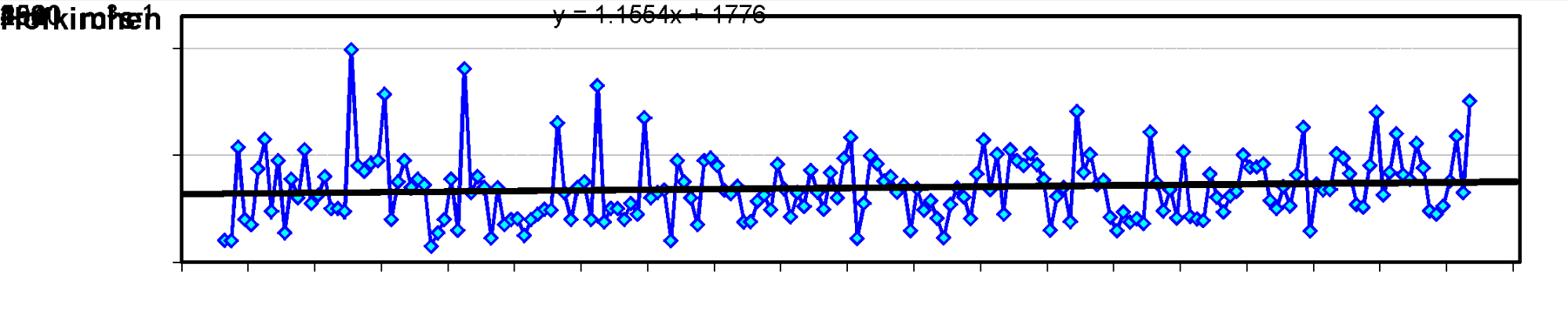
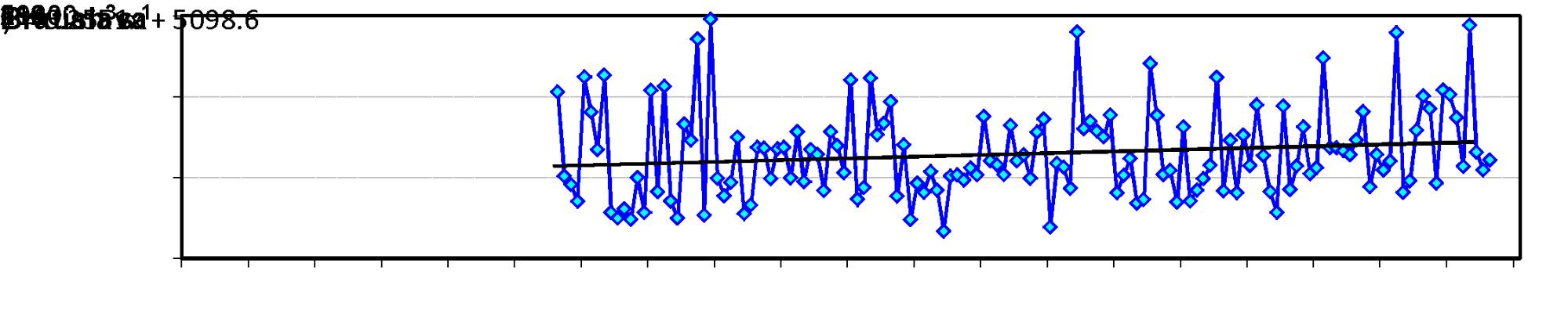
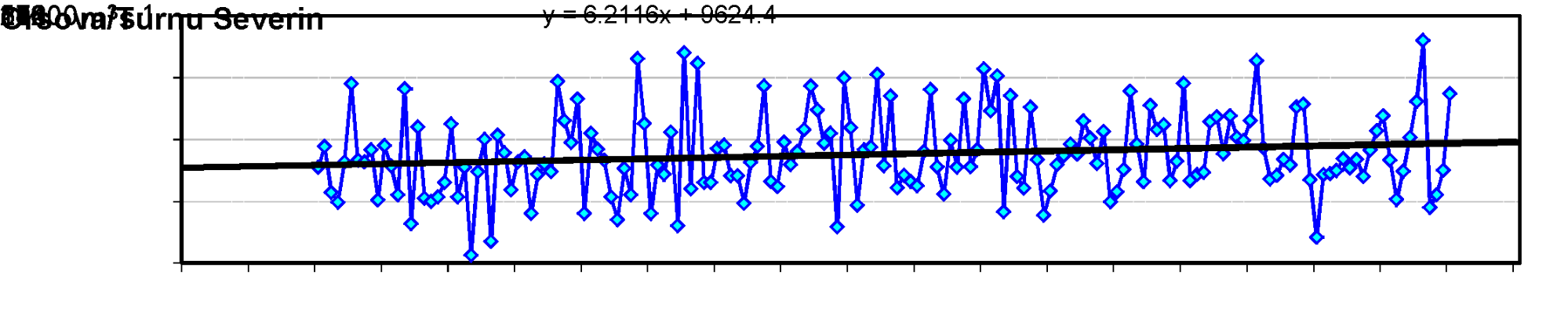
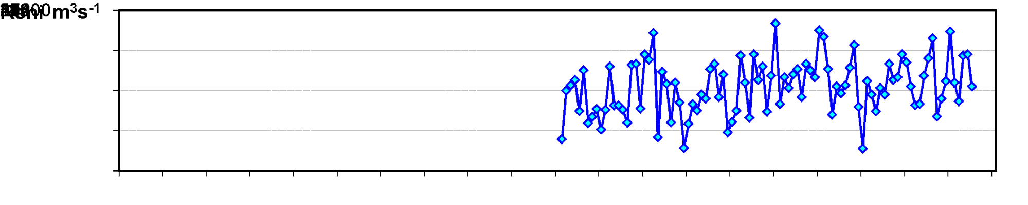
Fig. 3. The maximum annual discharges series

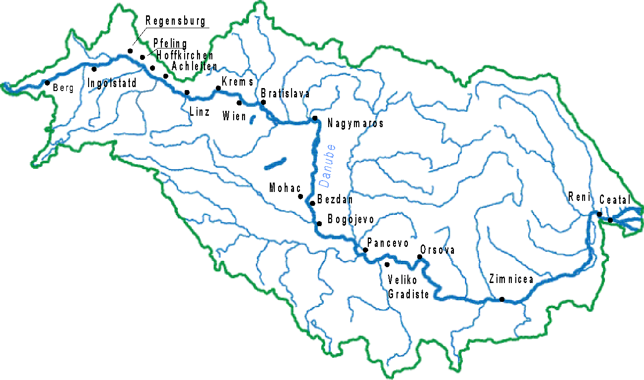
Fig. 4. Scheme of the Danube River basin and water gauging stations along the Danube River

Table 1. List of the gauging stations along the Danube River and Qamax – long-term average
of the maximum annual discharge

No.	River km	Gauge	Period	Country	Area [km2]	Elevation [m a.s.l.]	Mean Qmax [m3s-1]	Gw skew hist.
1	2613	Berg	1930–2007	GE	4047	489.48	204	-0.29
2	2458.3	Ingolstadt	1940–2007	GE	20001	359.97	1110	0.57
3	2376.1	Regensburg-Schwabelweis	1924–2007	GE	35399	324.06	1532	0.26
4	2300	Pfelling	1926–2007	GE	37757	307.73	1516	0.20
5	2256.9	Hofkirchen	1826–2013	GE	47496	299.17	1896	0.56
6	2150	Achleiten	1901–2007	GE	76653	287.27	4146	0.86
7	2135.2	Linz*	1821–2013	AT	79490	247.06	3670	0.60
8	2002.7	Stein-Krems (Kienstock)	1828–2006	AT	96045	193.32	5372	0.59
9	1934.1	Wien-Nussdorf*	1828–2006	AT	101731	157.0	5301	0.58
10	1868.8	Devin/Bratislava*	1876–2013	SK	131338	132.86	5884	0.24
11	1694.6	Nagymaros	1893–2007	HU	183534	99.37	5598	0.11
12	1446.8	Mohács	1930–2007	HU	209064	79.19	5063	0.04
13	1425.5	Bezdan	1940–2006	SR	210250	79.29	4974	0.30
14	1367.4	Bogojevo	1940–2006	SR	251593	76.11	5675	0.19
15	1153.3	Pancevo	1940–2006	SR	525009	65.98	10147	0.15
16	1060	Veliko Gradiste	1931–2007	SR	570375	60.83	10529	0.02
17	955	Orsova-Turnu Severin	1840–2006	RO	576232	44.76	10295	-0.19
18	554	Zimnicea	1931–2010	RO	658400	16.06	11087	-0.09
19	132	Reni	1921–2010	UKR	805700	0.2	11217	-0.40
20	72	Ceatal Izmail*	1931–2010	RO	807000	0.1	11173	0.02

*T-year discharges were estimated both including extreme historical data as well as excluding historical data from 1501, 1787 and 1897

RESULTS AND DISCUSSION

Estimation of the design values of the Qmax discharges along the Danube River

In this paragraph the design values for 20 gauge station along the Danube River were calculated. The Frequency curve spreadsheet version 3.06 (Dan Moor, August 2014) was used to estimate the parameters of distribution functions and to calculate the design values.

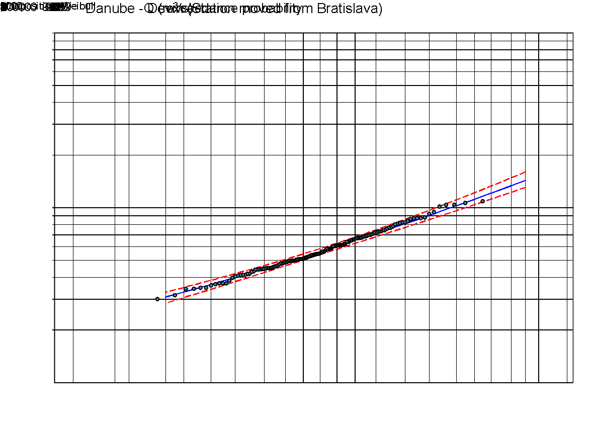
In the first step, we estimated the LP3 distribution function parameters (mean Q, standard deviation S, and station skewness coefficient G), for each of the stations separately and computed Qmax design values. In the case of gauges with historic floods, we added historic floods into the measured Qmax series (see Fig. 5), and recalculated the parameters of the distribution curves for individual stations having included the historic floods. The inclusion of the historical floods to calculation procedure has increased the skew coefficient Gh by 0.2 in average. The example for Danube: Bratislava station is presented in Fig. 6 a, b. Design values are sorted in Tables 2 a, b.

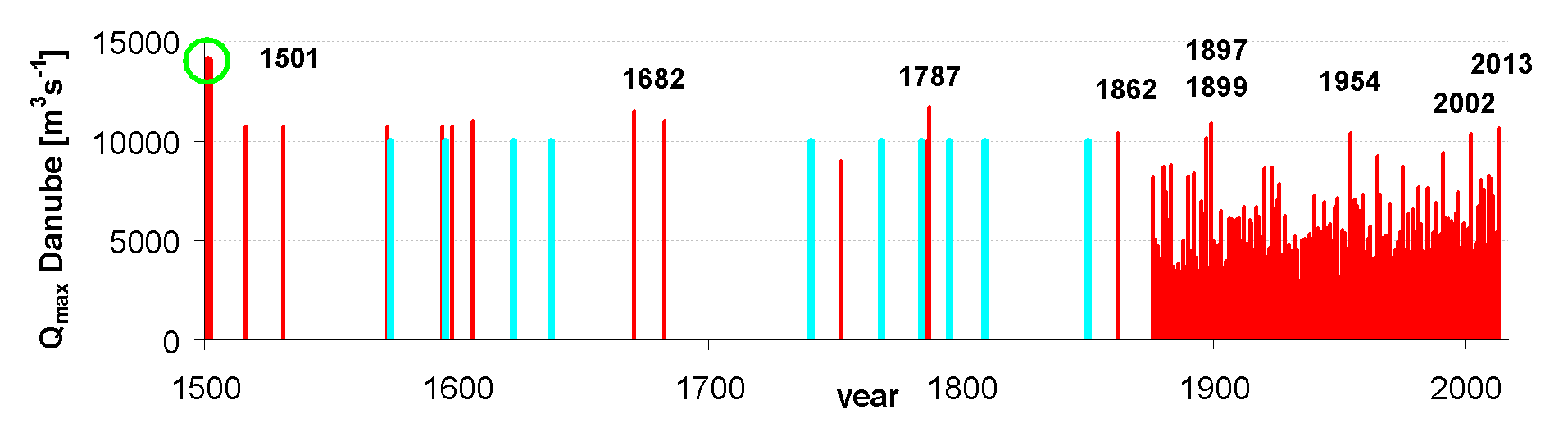
Fig. 5. Historical Danube River floods in river section Devín–Bratislava since 1500
up to 1876 (red columns - summer floods, blue columns - winter floods);
since 1876 - the observed annual peaks Qmax at the Bratislava water gauge

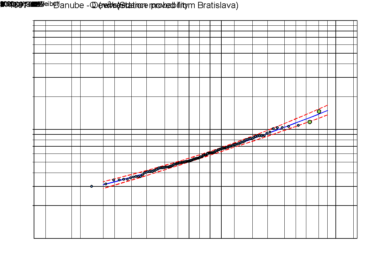
Fig. 6. Example of the computations output for the Danube at Bratislava/Devín station:
a) without historical data; b) with two historical data.
Distribution curve with confidence limits, design values

Tables 2a. Design values of selected T-year annual maximum discharges along the Danube River

River km	Station/T-year	5	10	50	100	200	500	1000
2613	Berg	272	324	432	476	518	573	613
2458.3	Ingolstadt	1327	1526	2002	2222	2453	2779	3043
2376.1	Regensburg-Schwabelweis	1902	2125	2530	2675	2809	2969	3081
2300	Pfelling	1888	2144	2649	2846	3034	3273	3447
2256.9	Hofkirchen	2334	2765	3840	4353	4905	5701	6359
2150	Achleiten	4839	5512	7155	7925	8744	9913	10869
2135.2	Linz	4641	5455	7352	8205	9092	10323	11304
2002.7	Stein-Krems (Kienstock)	6439	7397	9605	10592	11613	13028	14154
1934.1	Wien-Nussdorf	6345	7187	9046	9847	10658	11756	12610
1868.8	Devin/Bratislava	7129	8116	10273	11192	12119	13365	14328
1694.6	Nagymaros	6629	7325	8712	9257	9783	10457	10955
1446.8	Mohács	5958	6548	7708	8157	8589	9138	9541
1425.5	Bezdan	5807	6452	7847	8437	9029	9823	10435
1367.4	Bogojevo	6632	7334	8810	9418	10020	10815	11418
1153.3	Pancevo	11602	12611	14661	15483	16285	17326	18105
1060	Veliko Gradiste	12095	13128	15167	15962	16728	17708	18430
955	Orsova-Turnu Severin	11914	12901	14754	15445	16094	16901	17481
554	Zimnicea	12737	13776	15769	16528	17248	18155	18815
132	Reni	12963	13918	15596	16183	16715	17352	17793
72	Ceatal Izmail	12699	13677	15492	16161	16785	17557	18108
2b	With historic maxima
River km	Station/T-year	5	10	50	100	200	500	1000
2376.1	Regensburg-Schwabelweis*	1966	2298	3065	3407	3761	4249	4637
2300	Pfelling*	1964	2306	3089	3437	3795	4289	4680
2256.9	Hofkirchen*	2334	2765	3840	4353	4905	5701	6359
2150	Achleiten*	4995	5776	7748	8701	9730	11226	12472
2135.2	Linz*	4563	5453	7717	8818	10014	11758	13218
2002.7	Stein-Krems (Kienstock)*	6482	7535	10096	11295	12569	14384	15869
1934.1	Wien-Nussdorf*	6371	7329	9623	10682	11798	13374	14652
1868.8	Devin/Bratislava*	7166	8194	10479	11469	12476	13842	14909
1694.6	Nagymaros*	6671	7431	9020	9671	10314	11159	11799
132	Reni	12963	13918	15596	16183	16715	17352	17793
72	Ceatal Izmail*	12743	13830	15973	16808	17612	18640	19397

* With estimated historical maxima

Regionalization of the skew coefficients G for the stations along the Danube River

Firstly, the evaluation of several hydrological characteristics was analyzed along the Danube River. In Fig. 7 left there are presented course QT design values along the Danube. Development of the coefficients k=QT/Qa, (Qa is long term mean discharge) is presented in Fig. 7 right.

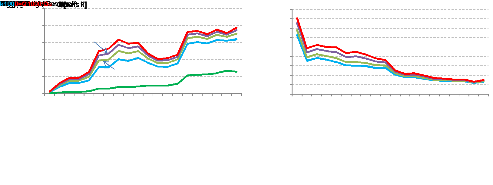
Fig. 7. Course of Q1000, Q500, Q200, Q100 design discharges, and Qa (left);
course of coefficient k1000, k500, k200, k100 (right) in stations along the Danube River

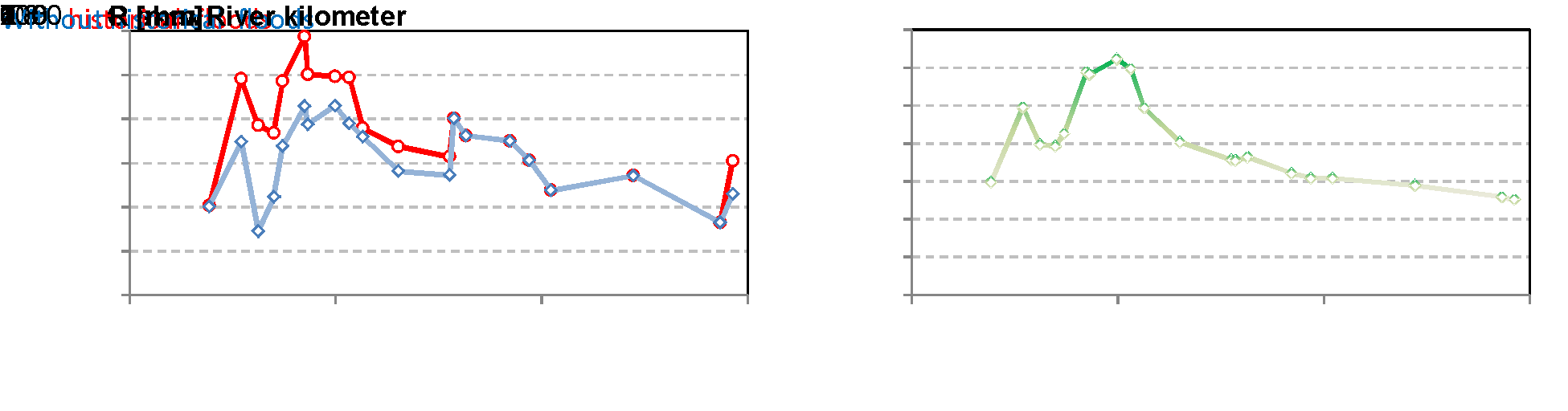
Fig. 8. Course of skew coefficients G and Gh (left) and course of runoff depth (right)
along the Danube River

The 1000-year discharge is 16-times higher than the mean annual discharge at station Berg, while only 7-times higher at station Bratislava, and only 3-times higher at station Reni.

From the Fig. 8 it follows, that the skew coefficients G and Gh have the similar course as long term runoff depth at the analyzed stations. Therefore, the following two best fitted relationships between the historical skew coefficient Gh and the runoff depth at the station were estimated:

Gh = 1.03437*ln(R) – 5.95 (11)

r² = 0.788;

Gh = 10.00246*R – 0.778 (12)

r² = 0.769;

where: R – long-term average annual runoff depth in mm (from 240mm to 640mm).

Finally, we propose to use the regional skew coefficient Gr calculated according to linear relationship (12) to estimate the T-year discharges in all stations on the Danube River.

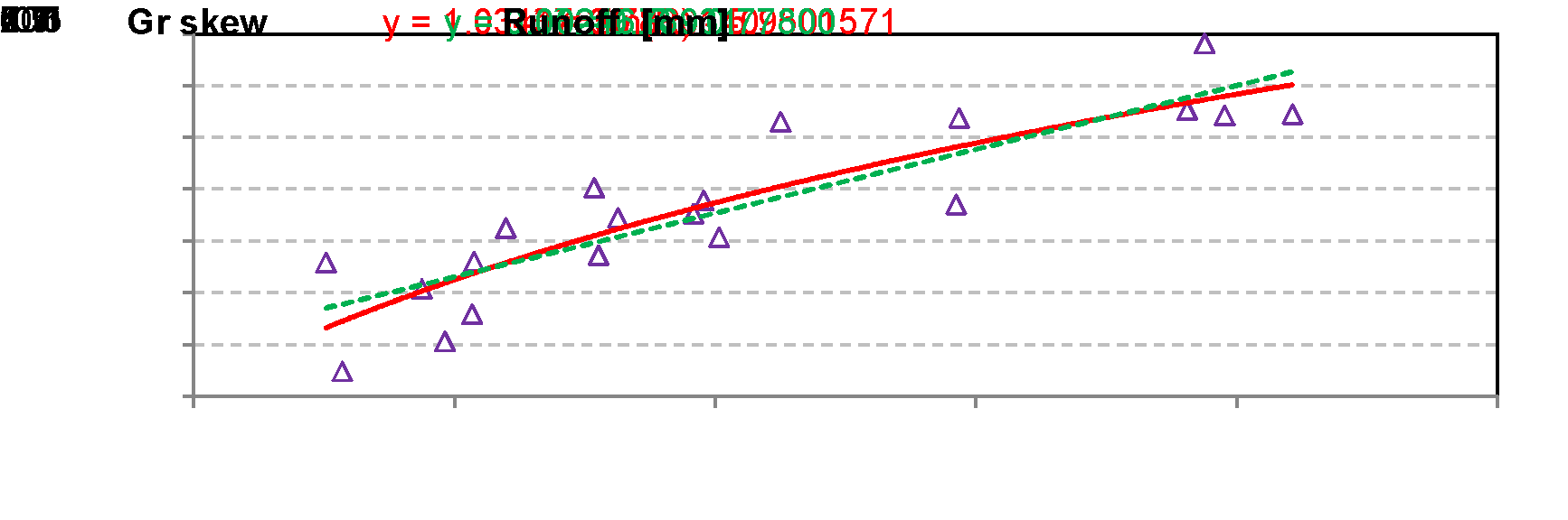
Fig. 9. Dependence of regional skew coefficient Gr on the runoff depth R, Danube River

CONCLUSION

With the increase of population – and with the development of civilization in general – an increase of vulnerability of the society is closely connected. It concerns also the threats by high floods as well as by incidents of long periods of droughts.

The territory of the Danube River is one of the most flood-endangered regions in Europe. Therefore, there is a strong need to have complete and exhausting information on the flood regime in order to be able to generalize such information on the basis of long-term observations from the whole Danube territory.

In estimating the extreme floods design values, we test the use of only one type of peak probability distribution, namely the log-Pearson type III distribution (LP3). This type of distribution is flexible and possible to reach extreme values according to coefficient of skewness (G). Coefficient of skewness calculated from measured data influences the shape of frequency curve. Steep slopes in catchments, low infiltrated areas, quick propagation of flood waves and one or more extremely high peak flows indicate high positive values of skewness (G). On the other hand, flat slopes, high infiltrated areas and runoff from catchment regulated by lakes and wetlands indicate negative values of skewness.

In the case of gauges with historic floods, we added historic floods into the measured Qmax series, and recalculated the parameters of the LP3 distribution curves for individual stations having included the historic floods. The inclusion of the historical floods to calculation procedure has increased the skew coefficient G to Gh by 0.2 in average. Historic coefficients of skewness (Gh) of the LP3 distribution curves are in a range from –0.404 to 0.861 along the Danube River.

For stations along the Danube River, we propose to apply the regional skew coefficient Gr, estimated according to relation (12). Using one type of distribution gives us a chance to generalize its skewness coefficients. Then we are able to estimate T-year discharges at gauges with short period of observations, and even between two observing gauges.

The calculated 1000-year discharge is 16-times higher than the mean annual discharge at station Berg, while only 7-times higher at station Bratislava, and only 3-times higher at station Reni.

The estimation of T-year discharges is never-ending process. Urbanization, channel regulation, flood protection construction and many other interventions, can change maximum discharges and negatively influence the application of frequency analysis. The future prediction of peak annual discharges is based on historical records. Land use changes and massive regulations of river beds can interrupt a stationarity of hydrological time series. Selected statistical variables (mean, median, skew, variation) have to be estimated appropriately from all the observing data. If anything will be changed in a catchment, it is necessary to recalculate distribution curves and define new T-year discharges in particular stations.

ACKNOWLEDGEMENTS

This study was supported by project VEGA 2/0009/15. Data used in study are from database of the MVTS project No. 9 ‘Flood regime of rivers in the Danube River basin” within the Regional co-operation of the Danube countries. Data from Ukraine were obtained in the framework of the Slovak-Ukrainian project: “Impacts of global climate change on water resources in Ukraine estimated by variability of river discharges and hydrograph components”. This publication is the result of the project implementation ITMS 26240120004 Centre of excellence for integrated flood protection of land supported by the Research & Development Operational Programme funded by the ERDF.

REFERENCES

Brazdil R., Kundzewicz Z.W., Benito G. Historical hydrology for studying flood risk in Europe, Hydrological Science Journal. 2006. 51(5). P. 739–764, DOI:10.1623/hysj.51.5.739.

Adler J.M. Danube Floodrisk. Manual of harmonized requirements on the flood mapping procedures for the Danube River, Data and methods. www.danube-floodrisk.eu, CESEP – Center for Environmental Sustainable Economic Policy. Bucharest, Romania. 2012. 95 p.

EC: Directive 2007/60/EC of the European Parliament and of the Council of 23 October 2007 on the assessment and management of flood risks, European Parliament, Council, 2007.

Elleder L. Reconstruction of the 1784 flood hydrograph for the Vltava River in Prague, Czech Republic. Global and Planetary Change. 2010. 70. P. 117-124.

Elleder L., Herget J., Roggenkamp T., Nießen A. Historic floods in the city of Prague – a reconstruction of peak discharges for 1481–1825 based on documentary sources. Hydrology Research. 2013. 44(2), P. 202-214.

Gaal L., Szolgay J., Kohnova S., Hlavcova K., Viglione A. Inclusion of historical information in flood frequency analysis using a Bayesian MCMC technique: A case study for the power dam Orlik, Czech Republic. Contributions to Geophysics and Geodesy. 2010. 40(2), P. 121-147.

Griffis V.W., Stedinger J.R. The log-Pearson type III distribution and its application in flood frequency analysis. 1: Distribution characteristics. Journal of Hydrologic Engineering. 2007. 12(5). P. 482-491.

Griffis V.W., Stedinger J.R. Log-Pearson type 3distribution and its application in flood frequency analysis, III—sample skew and weighted skew estimators. Journal of Hydrology. 2009. 14(2). P. 121-130.

Hirsch J. Probability plotting position formulas for flood records with historical information. Journal of Hydrology. 1987. 96(1-4). P. 185-199. https://doi.org/10.1016/0022-1694(87)90152-1

Hirsch R.M., Stedinger J. Plotting Positions for Historical Floods and Their Precision. Water Resources Research. 1987. 23(4). P. 715-727. DOI: 10.1029/WR023i004p00715

Cheng K.S. Chiang J.L., Hsu C.W. Simulation of probability distributions commonly used in hydrological frequency analysis. Hydrological Process. 2007. 21(1). P. 51-60.

IACWD. Guidelines for determining flood flow frequency. Bulletin 17-B. Technical report, Interagency Committee on Water Data, Hydrology Subcommittee. 1982. 194 p.

ICPDR. The Danube River Basin District, Part A – Basin-wide overview. ICPDR Document IC/084, Vienna, 2005. 175 p.

ICPDR. Danube River Basin District Management Plan, Part A – Basin-wide overview. ICPDR Document number: IC/151, Vienna, 2009. 91 p.

ICPDR. Flood Risk Management Plan for the Danube River Basin District. ICPDR, Vienna, 2015. 77 p.

Kjeldsen T.R., Macdonald N., Lang M., Mediero L., Albuquerque T., Bogdanowicz E., Brazdil R., Castellarin A., David V., Fleig A., Gul G. O., Kriauciuniene J., Kohnova S., Merz B., Nicholson O., Roald L.A., Salinas J.L., Sarauskiene D., Sraj M., Strupczewski W., Szolgay J., Toumazis A., Vanneuville W., Veijalainen N., Wilson D. Documentary evidence of past floods in Europe and their utility in flood frequency estimation. Journal of Hydrology. 2014. 517. P. 963-973. ISSN 0022-1694. DOI: http://doi.org/10.1016/j.jhydrol.2014.06.038

Koutsoyiannis D. Uncertainty, entropy, scaling and hydrological statistics. Hydrological Sciences Journal. 2005. 50(3). P. 381-404.

Laszloffy W. (1965) Die Hydrographie der Donau. Der Fluss als Lebensraum. In: Liepolt, R. (ed.): Limnologie der Donau – Eine monographische Darstellung. II. Kapitel, Schweizerbart, Stuttgart. P. 16-57.

Merz R., Blöschl G. Flood frequency hydrology: 1. Temporal, spatial, and causal expansion of information, Water Resources Research. 2008a. 44(8). W08432. DOI: 10.1029/2007WR006744

Merz R., Blöschl G. Flood frequency hydrology: 2. Combining data evidence. Water Resources Research. 2008b. 44(8). W08433. DOI: 10.1029/2007WR006745

Merz B., Kreibich H., Thieken A., Schmidtke R. Estimation uncertainty of direct monetary flood damage to buildings. Nat. Hazards Earth Syst. Sci. 2004. 4. P. 153-163, https://doi.org/10.5194/nhess-4-153-2004

Pilon, P.J., Adamowski, K. Asymptotic variance of flood quantile in log Pearson type III distribution with historical information. Journal of hydrology. 1993. 143 (3-4). P. 481-503.

Rogger M., Kohl B., Pirkl H., Viglione A., Komma J., Kirnbauer R., Merz R., Blöschl G. Runoff models and flood frequency statistics for design flood estimation in Austria – Do they tell a consistent story? Journal of Hydrology. 2012. 456-457. P. 30-43.

Stănescu V.A. Regional analysis of the annual peak discharges in the Danube catchment. Follow-up volume No.VII to the Danube Monograph. Regional Cooperation of the Danube Countries. Bucuresti Institutul Naional de Hidrologie si Gospodarie a Apelor Bucuresti. Bucharest. 2004. 64 p.

Stancik A., Jovanovic S. et al. Hydrology of the River Danube. Priroda Publishing House. Bratislava. 1988. 271 p.

Stedinger J. R., Griffis V.W. Flood Frequency Analysis in the United States: Time to Update. Journal of Hydrologic Engineering. 2008. 13(4). P. 199-204.

Szolgay J., Kohnova, S., Hlavcova, K. Uncertainties of Estimating Design Floods. Environment. 2003. 37(4). P. 194-199 [in Slovak].

Back to CONTENTS

ASSESSMENT HARMONIZATION PROBLEMS OF THE LONG RETURN PERIOD FLOODS ON THE DANUBE RIVER